


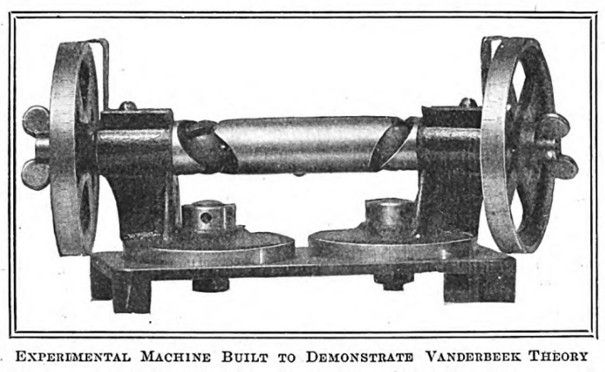
Already in 1908, there was a need in understanding the kinematical relations of universal joints. This Motor Age article shows an analysis of the kinematic relations that have to be accounted for, applying a universal joint. It becomes clear, that by pairing two universals via an intermediate shaft, what requirements are necessary to assure a less speed variation as possible between driver and driven one.
.
Text and jpegs by courtesy of hathitrust.org www.hathitrust.org, compiled by motorracinghistory.com
Motor Age, Vol. XIV (14), No. 15, October 8, 1908
THE LIMITATIONS OF THE UNIVERSAL JOINT
By H. Vanderbeek
ALTHOUGH the universal A joint, originally known as Hooke’s coupling, has been widely used for feed mechanisms on machine tools, for driving drill spindles, and in agricultural machinery, it was not generally employed for the transmission of considerable powers until the advent of the bevel-gear-driven-rear-axle motor car. Fundamentally, the universal joint is a device for the transmission of rotary motion between two shafts whose axes intersect in a point, with varying angles with each other; and although modified forms of the device are made which allow for lateral displacement of the axes, it is the purpose of the writer to analyze the operation, and determine the peculiarities and limitations of the universal joint in its true form; the modifications must necessarily be considered as individual cases, and are outside the scope of this article.
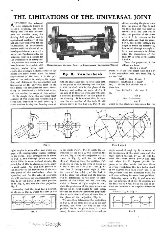
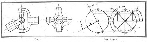
In its simple form, the universal joint consists of two shaft-ends terminating in forks and connected to each other by a cross member having two bearing axes at right angles to each other and which engage with corresponding journal bearings in the forks. This arrangement is shown in Fig. 1, and although joints are made which differ in constructional details, the principles of this fundamental form apply in most cases. We will now proceed to the analysis of the movements of the several parts of the mechanism, when in operation, and for the sake of clearness, we will construct the diagrammatic view, Fig. 2, of the parts in the same position as in Fig. 1, and also the side projection Fig. 3.
Assuming that the joint has a position as shown in Fig. 1, where the fork B lies with its shaft axis and its cross axis both in the plane of the drawing and the fork A with its shaft axis in the plane of the drawing, and making an angle of θ with the axis of B, then the cross axis will have a position perpendicular to the plane of the drawing. It is evident that in rotation the extremities of the fork B will always move in the line c-e, Fig. 2, and in the circle c‘-g-e‘-i, Fig. 3, while the extremities of the fork A will describe the line b-a, Fig. 2, and the projection of this trace, in Fig. 3, will be the ellipse, i-b‘-g-a‘. Starting from the position, c‘-e‘, as shown in Fig. 3, the fork B being at c‘ and e‘ and the fork A at i and g, we turn fork B through some angle ẞ, then the trace of the point i, of the fork A will be along the ellipse and its location will be determined by the point of intersection of the ellipse and the line o-m, which is drawn at right angles to o-m‘, since the projection of the cross axes must always be at right angles to each other, because the axes are themselves perpendicular to each other and one of them lies in the plane of the projection, Fig. 3.
We have then determined the projection, in Fig. 3, of the cross axis of A in its new position, but since this line in its true position lies in the plane b-o-a, it is necessary, in order to determine its actual position, to swing the plane b-o-a into the plane of Fig. 3, and we then find that the point h travels to k, and that o-k is the true position of the cross axis of A in relation to its shaft axis, and that the member A has moved through an angle β while the member B, has moved through an angle β. It is now necessary to determine the dimensions of the angle Ω* in terms of the angles ẞ and θ.
From the properties of the ellipse we know, fk : fh :: oi : o-b‘ where oi is the semi-major axis and o-b‘ is the semi-minor axis, and from Fig. 3, we see that fk : fh :: tan Ω : tan β
therefore: tan Ω : tan β :: oi : ob‘
but, oi = Ob and ob‘ = ob cos θ
therefore tan Ω : tan ß :: ob cos θ or tan Ω = tan β / cos θ.
which is the algebraic expression for the angle moved through by B, in terms of the inclination of the shaft axes and the angle moved through by A. It will be noted that when 2=0 B=0 and also that when 2=90 degrees β=90 degrees, or in other words, that four times in every revolution, the two forks stand at 90 degrees with each other, and it is also, evident that the maximum variation will occur midway between these positions.
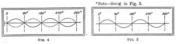
Referring again to Fig. 3, and continuing the rotation of B for 90 degrees, we see that o-n of A will be at o-n‘ and is be- hind the member A an angular difference equal to the amount it was in advance in the former position, or in other words, its angular position is now negative while it was positive before. The angular position must not here be confused with the angular velocity. From what we have seen we may conclude that this same angular relation is repeated in the two remaining quadrants of the cycle, and we may plot these relative positions as shown in Fig. 4.
In practical application of the above, the maximum angular variation between the two members is probably of more interest than the angular velocity ratio, and in order to present this variation in concrete form, the following table will be of value:
(table Angle between shaft axes – Maximum angular variation – Length of arc, of circle of 3″ diameter).
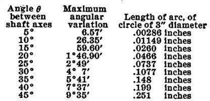
The angular variation and the length of the arc in the above are given as the numerical difference, which occurs both positively and negatively, twice in every revolution.
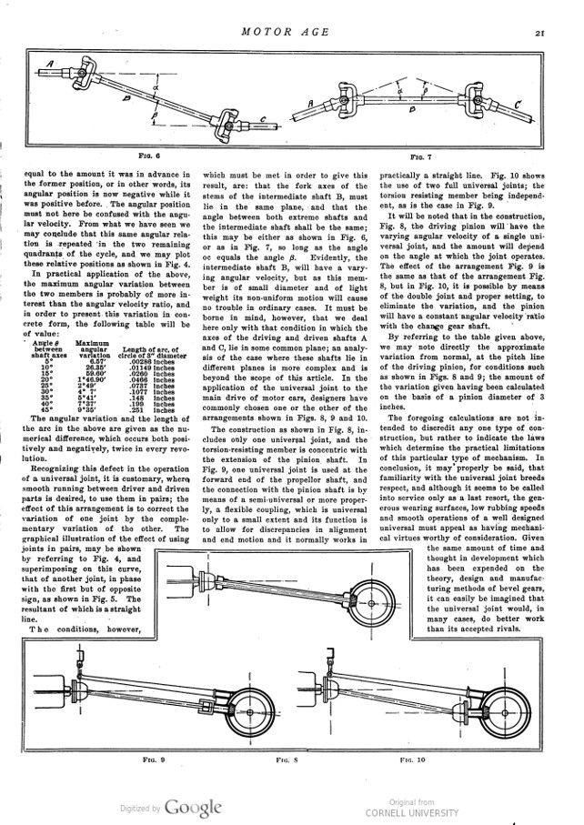
Recognizing this defect in the operation of a universal joint, it is customary, where smooth running between driver and driven parts is desired, to use them in pairs; the effect of this arrangement is to correct the variation of one joint by the complementary variation of the other. The graphical illustration of the effect of using joints in pairs, may be shown by referring to Fig. 4, and superimposing on this curve, that of another joint, in phase with the first but of opposite sign, as shown in Fig. 5. The resultant of which is a straight line.
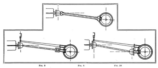
The conditions, however, which must be met in order to give this result, are: that the fork axes of the stems of the intermediate shaft B, must lie in the same plane, and that the angle between both extreme shafts and the intermediate shaft shall be the same; this may be either as shown in Fig. 6, or as in Fig. 7, so long as the angle oc equals the angle β. Evidently, the intermediate shaft B, will have a varying angular velocity, but as this member is of small diameter and of light weight its non-uniform motion will cause no trouble in ordinary cases. It must be borne in mind, however, that we deal here only with that condition in which the axes of the driving and driven shafts A and C, lie in some common plane; an analysis of the case where these shafts lie in different planes is more complex and is beyond the scope of this article. In the application of the universal joint to the main drive of motor cars, designers have commonly chosen one or the other of the arrangements shown in Figs. 8, 9 and 10.
The construction as shown in Fig. 8, includes only one universal joint, and the torsion-resisting member is concentric with the extension of the pinion shaft. In Fig. 9, one universal joint is used at the forward end of the propellor shaft, and the connection with the pinion shaft is by means of a semi-universal or more properly, a flexible coupling, which is universal only to a small extent and its function is to allow for discrepancies in alignment and end motion and it normally works in practically a straight line. Fig. 10 shows the use of two full universal joints; the torsion resisting member being independent, as is the case in Fig. 9.
It will be noted that in the construction, Fig. 8, the driving pinion will have the varying angular velocity of a single universal joint, and the amount will depend on the angle at which the joint operates. The effect of the arrangement Fig. 9 is the same as that of the arrangement Fig. 8, but in Fig. 10, it is possible by means of the double joint and proper setting, to eliminate the variation, and the pinion will have a constant angular velocity ratio with the change gear shaft.
By referring to the table given above, we may note directly the approximate variation from normal, at the pitch line of the driving pinion, for conditions such as shown in Figs. 8 and 9; the amount of the variation given having been calculated on the basis of a pinion diameter of 3 inches.
The foregoing calculations are not intended to discredit any one type of construction, but rather to indicate the laws which determine the practical limitations of this particular type of mechanism. In conclusion, it may properly be said, that familiarity with the universal joint breeds respect, and although it seems to be called into service only as a last resort, the generous wearing surfaces, low rubbing speeds and smooth operations of a well-designed universal must appeal as having mechanical virtues worthy of consideration. Given the same amount of time and thought in development which has been expended on the theory, design and manufacturing methods of bevel gears, it can easily be imagined that the universal joint would, in many cases, do better work than its accepted rivals.